Chapter 16 Finding Prospects

Prospect identification is one of the most common uses of descriptive and predictive analytics in fundraising, especially for direct mail appeals.

Whether you are acquiring new donors or reactivating former donors, identifying prospects and creating prioritized segments for direct response marketing efforts makes financial sense. For example, as we saw in Figure 1.2, if we can improve the response rate of a direct mail appeal and simultaneously reduce the number of target recipients, we can expect to generate, on average, more revenue while also reducing overall mailing costs (Bult, Van der Scheer, and Wansbeek 1997).

There are many ways to experiment with prospect segmentation to increase efficiency and revenue for direct mail appeals. The following are two common methods.

Select a target list of prospects based on giving likelihood
Upgrade the ask amount in an appeal based on predicted gift size

First, let’s establish a general framework for defining prospect segments. Next, we will explore a couple use cases which describe how to use predictive analytics to create prospect segments and increase results.

16.1 Prospect Segments

Prospect segmentation involves organizing prospects into segments (groups) based on a variety of prospect attributes. One common approach is to organize prospects into a prospect quadrant defined by any two prospect characteristics such as gift capacity versus giving likelihood.

In the Data Visualization chapter, we provided a recipe to create an example text plot that displays prospects with wealth ratings of $1,000,000–$2,499,999, along with their major giving likelihood. Now, imagine a quadrant plot that displays prospects for all wealth ratings (low to high) relative to their giving likelihood. Similarly, imagine a quadrant plot that displays prospect event attendance frequency relative to their predicted gift size.

The following prospect quadrant provides a general framework for organizing prospects according to various attributes to create different segments.

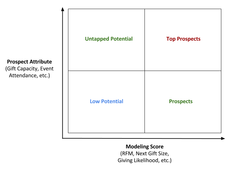
FIGURE 16.1: Prospect quadrant

Intuitively, the prospects with the highest gift capacity and giving likelihood values will typically represent the top prospects for your organization. Similarly, the prospects with highest event attendance and RFM score will often represent your top prospects. By organizing your prospects into different segments, you can identify prospect recommendations and prioritize different actions for each group.

For example, if you have prospects with high giving likelihood and low financial capacity, then you may decide to directly solicit this group, but adjust the solicitation amounts based on their gift capacity. Likewise, if you have prospects with high capacity and low giving inclination, you may opt to pursue peer-based solicitation rather than a direct mail approach. For low potential prospects with low gift capacity and low affinity scores, you may opt to send them a web-based survey to gauge interest or invite them to an upcoming event to learn more about your organization or cause. For the top prospects with high giving likelihood and high financial capacity, you may opt to send a highly personalized introduction appeal to a subset of this group and exclude the other portion of this group—perhaps based on prospect management or demographic attributes—in favor of individual outreach from a gift officer.

Ultimately, all of these examples reflect the importance of tailoring your solicitation and outreach approaches by using important prospect signals (descriptive indicators, predictive scores, etc.) available in your donor data. Regardless of your approach, it is critical that you track, monitor and analyze your results to continuously improve your donor outreach efforts.

16.2 RFM

RFM remains a popular choice for prospect segmentation and direct response marketing efforts due to its familiarity and ease of use. In the RFM Modeling chapter, we explore multiple use cases for RFM scores and ranking, including finding donors, upgrade donors, lapsed donors, etc. If you are newer to fundraising, we recommend you explore RFM scores and identify new ways you can creatively apply this simple method to your own fundraising problems.

16.3 Giving Velocity

Giving velocity is an index that measures the rate of change in donor giving over a specific length of time. Similar to RFM, the premise is to analyze giving histories for comparative insight at the individual donor level. Giving velocity is useful for identifying donors whose change (trend) in giving has significantly increased within recent years. High degrees of positive variation in recent giving may be indicative of a significant change in wealth capacity (for example, due to a recent liquidity event). To learn more about giving velocity, check out this article.

The concept of giving velocity, as well as other RFM modeling variations, has been a popular topic of discussion on the Prospect-DMM forum. Prospect-DMM is a free, online discussion group you can join to connect with other development professionals who are interested in data mining and modeling (often with a focus on major gifts). You can access and sign up for the Prospect-DMM email group via this site.

16.5 Gift Capacity and Inclination

Gift capacity and inclination are two fundamental attributes included in most CRM databases, prospect reports, and products today, which includes wealth screening services and propensity modeling tools. Gift capacity and inclination attributes are useful and prevalent because they help identify whether a prospect has the means (capacity) and inclination (likelihood) to support your organization or cause.

Based on these two factors, we can revise our general prospect quadrant and propose some example recommendations based on each segment.

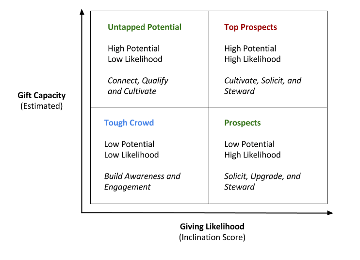
FIGURE 16.2: Gift capacity versus giving likelihood

Gift capacity and inclination are indeed useful attributes for prioritizing your prospects, but they are only part of the picture. Let’s explore some additional attributes you can use to better understand your prospects in the context of your institution.

16.6 Engagement Scores

Affinity, connection and engagement scores remain a popular topic within the fundraising community. Why? Because giving capacity and inclination scores alone do not necessarily translate to a gift if the prospect lacks awareness, emotional engagement or a meaningful connection to your institution.

Today’s donors are savvy and, with more than 1.5 million nonprofit organizations registered in the U.S. according to the National Center for Charitable Statistics (NCCS), institutions have to compete for donor’s time, attention, and commitment.

Given this reality, many development organizations have shifted, or have begun shifting, towards a more holistic prospecting approach that integrates traditional indicators, such as giving capacity and inclination (giving likelihood or propensity), with relationship-focused measures, qualities and appraisals such as degree of activity, engagement, and affinity. Similar to the previous attributes, we can update our general prospect quadrant to organize prospects by financial capacity and depth of engagement (perhaps using proxy measures such as volunteer involvement, event attendance frequency, etc.).

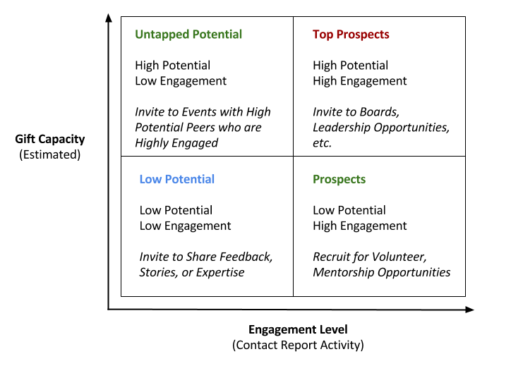
FIGURE 16.3: Gift capacity versus engagement

Now that we have explored some basic prospect segmentation concepts, let’s explore a couple use cases of how you can use prospect segments to define solicitation groups as well as upgrade pathways.

16.7 Annual Giving

Annual giving plays an important role in any organization’s fundraising efforts to broaden its donor base and strengthen its level of regular financial support.

In the short term, annual giving programs tend to focus on increasing revenue through various donor-centric engagement and annual solicitation activities. In the long term, annual giving programs often seek to build a sustainable pipeline of new donors (acquisition), who repeatedly or consistently give (retention), and over time increase their level of support (upgrade) to major gifts through multi-year pledges or planned giving options such as bequests.

The definition of major gift size varies by institution and depends on multiple factors such as existing levels of philanthropic support, current number of donors, and major gift capacity.

Annual giving programs can use multiple methods and channels to promote institutional awareness, show impact, and solicit support, including:

Direct mail
telefund
E-solicitations
Online giving
Mobile and text-based giving
Giving days
Crowdfunding
Face-to-face solicitations
Volunteer or peer-based solicitations

For additional information on annual giving campaign fundamentals, check out this CASE resource.

For this annual giving example, we will assume you’ve already worked through the regression examples in the Machine Learning Recipes and Predicting Gift Size chapters.

Let’s explore how to segment and upgrade the ask amounts in annual giving appeals based on predicted gift size. For this example, we will define annual gift size as gifts below $25,000.

The following is some example pseudocode to load your own data.

# Load readr
library(readr)

# Load dplyr
library(dplyr)

# Load Data
donor_data <- read_csv("data/YourDataFile.csv")

# Select variables
donor_data <- select(
 donor_data,
 pred_vars,
 TotalGiving)

# Convert features to factor
donor_data <- mutate_at(donor_data,
  .vars = pred_vars,
  .funs = as.factor)

Now that your data is loaded and prepared, let’s suppose you decide to build a multiple linear regression model to predict gift size.

# Fit multiple linear regression model
giving_mlg_model <- lm(TotalGiving ~ ., 
  data = donor_data)

Next, let’s store the numerical predictions.

donor_data$TotalGiving_pred_mlg <- predict(giving_mlg_model)

Based on our example definition of annual gift size, let’s build a list of annual giving-level donors.

annual_giving_list <- filter(donor_data, 
  CurrFYGiving_pred_mlg < 25000)

Assuming we have limited resources for a direct response marketing project, let’s create targeted annual giving solicitation segments using predicted gift sizes as segment criteria:

E-solicitation segment for predicted gift size of $1-$49
Postcard solicitation for predicted gift size of $50-$99
Direct mail solicitation for predicted gift size of $100 to $499
Color brochure solicitation for predicted gift size of $500 and above

# Create e-solicitation segment
annual_giving_esol <- filter(annual_giving_list, 
  CurrFYGiving_pred_mlg > 1 & CurrFYGiving_pred_mlg < 50)

# Create postcard segment
annual_giving_postcard <- filter(annual_giving_list, 
  CurrFYGiving_pred_mlg > 50 & CurrFYGiving_pred_mlg < 100)

# Create direct mail segment
annual_giving_dmail <- filter(annual_giving_list, 
  CurrFYGiving_pred_mlg >= 100 & CurrFYGiving_pred_mlg < 500)

# Create color brochure segment
annual_giving_cbrochure <- filter(annual_giving_list, 
  CurrFYGiving_pred_mlg >= 500)

As long as you create segments with prospects IDs for your different annual giving solicitations, you can later monitor and measure the response rate and total giving for each segment. A simple way to compare the results is to use a table, as shown in Table 16.1.

TABLE 16.1: Annual giving mailing segments example
Group	Size	Cost	Gifts received	Gift total	Net revenue
E-solicitation	4000	$0	185	$1,825	$1,825
Postcard	1000	$500	58	$1,814	$1,314
Direct mail	500	$500	27	$2,750	$2,250
Leadership brochure	100	$500	3	$2,500	$2,000

In this example, we used predicted gift size to create annual giving segments and make annual giving upgrade solicitation recommendations. Using past giving data, we learned how to build a mockup regression model and use gift size predictions to select annual giving collateral. Specifically, we chose lower-cost solicitation methods for smaller gift size predictions and reserved more expensive print materials for larger gift sizes.

Build a classification model that predicts annual giving likelihood using your own data. Also build a regression model that predicts annual gift size. Using both giving likelihood and predicted gift size, can you identify your top predicted annual giving donor segments?

16.8 Planned Giving

Calculating the return or ROI (return on investment) on planned giving appeals or mailing requests for more information is a difficult problem. Why? Simple reasons: 1) making a planned gift is a complex “stop and think” decision, which usually requires legal and financial consultation and spousal discussion if married; and 2) there’s a long delay between a person receiving an appeal and an organization receiving a gift. Nevertheless, we still can come up with a list of prospects that will likely have a higher response rate on average. Let’s see how.

As you prepare your planned giving appeal, you will no doubt face the question “should I create separate lists or mailings for different planned giving options?” While this is a reasonable question, you may find that you have small sample sizes for each type of planned gift (for example, bequests, life income gifts, gift annuities, and charitable remainder trusts), which can make it difficult to make accurate planned giving predictions.

When building your own planned giving models, you may find that your classification models are less likely to overfit if you try to predict a “planned gift donor” outcome instead of a “charitable remainder trust” donor.

We recommend that you first focus your efforts on an overall higher response rate for a “request for more information” type of planned giving mailing. You will get highly qualified leads this way.

With the rise of computational advertising, there’s also the option of buying Facebook ads to target people who are highly likely to make a planned gift through online giving vehicles. Regardless of the option you choose, you should include a test and a control group for targeting purposes.

As you review and finalize your planned giving appeal, your planned gift officers may tell you that planned gift donors are typically older and have no children. This makes an excellent selection criterion to test response.

We encourage you to conduct descriptive and exploratory analysis on your own planned giving data to identify giving likelihood and age values that are practical and make sense for your target audience, especially since your predictive scores and demographics will vary relative to your institutional donor base and record of giving activity.

For the rest of this use case, we will assume that you already read the Machine Learning Recipes chapter and built your own planned giving model to generate giving likelihood scores for each constituent in your test dataset.

The following is some example pseudocode to load the planned giving scores you built.

library(reader)
library(dplyr)

donor_data <- read_csv("data/YourDataFile.csv")

Although based on probability, any person with a score of about 50 is a good planned giving prospect; for a higher response rate, we will select prospects with a score of 80 and above. Of course, we need to exclude current planned giving donors.

planned_giving_list <- filter(donor_data, 
                              pg_score > 80 & 
                                pg_donor_ind == 'N')

Let’s suppose we have the budget to send a brochure to about 6,000 people. We can select 5,000 using the predictive scores and 1,000 using common knowledge. This doesn’t meet the statistical need of comparable sample sizes, but let’s stick to this example. If you have resources and buy-in from your planned giving office, feel free to draw different sample sizes.

planned_giving_list_test <- top_n(planned_giving_list, 
                                  n = 5000, 
                                  wt = pg_score) %>%
  mutate(group = 'test')

Let’s select the control group.

planned_giving_list_control <- filter(donor_data, 
                                      pg_score < 81 & 
                                        pg_donor_ind == 'N' & 
                                        age > 60) %>% 
  sample_n(size = 1000) %>% 
  mutate(group = 'control')

Let’s combine them.

planned_giving_final_list <- bind_rows(planned_giving_list_test, 
                                       planned_giving_list_control)

As long as you have this list with the IDs of the prospects in both the groups, you can later calculate the response rate for each group. A simple way to compare the results is to use a table, as shown in Table 16.2.

TABLE 16.2: Test results from a mailing
Group	Size	Responses	Gifts received	Gift amount
Control	1000	20	5	$100,000
Test	5000	100	20	$500,000

In this planned giving example, we explored how to select a target list of prospects based on your own giving likelihood scores. Next, we outlined how to construct a test and control group of planned giving prospects using the example criteria of giving likelihood scores of 80 and above and age values greater than 60 years old.

Once the planned giving mail solicitation is delivered to your target audience, you should monitor and measure the response rates over a certain time period in consultation with your planned giving team. If your predictive model is doing its job, you should expect to see a higher response rate from the test group based on your predicted response estimates.

16.9 Summary

In this chapter, we discussed the role of prospect segmentation in donor solicitation and outreach efforts. We explored how to use descriptive and predictive methods to find prospects for a variety of use cases, including annual giving and planned giving. Building on the Machine Learning Recipes, Predicting Gift Size, and Social Network Analysis chapters, this chapter focused on applying some of these methods to finding prospects and creating segments to increase efficiency and fundraising revenue.

After reading this chapter, we hope you are inspired to further explore your fundraising problems and apply machine learning methods to your institutional data to identify actionable insights, generate recommendations, and create experiments with measurable outcomes.

In the next chapter, we will explore some important new trends, technology, and applications designed to tap into organizational data to uncover useful patterns that translate to decision support, recommendations and, ultimately, organizational knowledge.

References

Bult, Jan Roelf, Hiek Van der Scheer, and Tom Wansbeek. 1997. “Interaction Between Target and Mailing Characteristics in Direct Marketing, with an Application to Health Care Fund Raising.” International Journal of Research in Marketing 14 (4). Elsevier: 301–8.