Chapter 11 RFM Modeling
Recency, Frequency, Monetary (RFM) modeling has its root in direct marketing. Although many sophisticated statistical techniques were developed after the initial use of RFM, it remains a top choice for marketers to segment their population (McCarty and Hastak 2007). The ease of use of RFM models is the primary reason for its widespread use (Verhoef et al. 2003). Secondly, as we saw in Section 3.2, since the decision-makers understand the segments based on RFM easily, they are more likely to use them. Some researchers have argued that its simplicity goes against the efficiency of other models (A. X. Yang 2004). Taking note of that argument, we will look into how to develop our own RFM models.
11.1 Calculate RFM Values
Let’s review the definitions of RFM.
- Recency measures how recently the customers (in our case, donors) made a transaction.
- Frequency measures how often the customers make transactions.
- Monetary measures how much money that the customers spent on their transactions.
As you can guess, a donor who made a recent gift, has been giving frequently, and makes large gifts is likely to make further gifts. Of course, there are quite a few parameters at play here. Let’s denote the low values for each of the measures with a negative sign and the high values with a positive sign.
What do you think of the following donors?
- R- F+ M+: It has been a while since they gave but they gave frequently and gave a lot. Did we lose them?
- R+ F- M-: They gave recently but have not given frequently and not a whole lot. Are these new donors?
- R+ F- M+: They gave recently but have not given frequently. They made some big gifts. Did we get lucky with these donors?
If you just use two values (that is, high or low), you will have eight combinations of RFM to go through—many opportunities for segmentation! How you use these scores depend on your objective: Do you want to upgrade donors or do you want to save mailing costs? Before you compute these scores, you must decide what recent means. Is it the last month or last year?
All right. Let’s write some code to get our RFM values. Most likely you will pull the data for this analysis from a transactional table. The common format of such a table includes multiple rows per donor per gift. Table 11.1 shows an example:
| DONOR_ID | GIFT_DATE | GIFT_AMOUNT |
|---|---|---|
| 3 | 2017-01-30 | $5,803.17 |
| 4 | 2017-03-04 | $6,602.89 |
| 6 | 2017-01-02 | $7,327.90 |
| 6 | 2017-02-12 | $8,662.71 |
| 8 | 2017-06-18 | $5,947.82 |
We need to transform this data to summarize recency, frequency, and monetary data for each donor, creating one row per donor. You will find the sample data file with gift transactions in the code bundle for this book. Let’s read this data first.
library(readr)

rfm_data <- read_csv("data/SampleDataRFM.csv")

head(rfm_data)
#> # A tibble: 6 x 3
#>      ID FISCAL_YEAR Giving
#>   <int>       <int>  <chr>
#> 1     1        2015 $1,000
#> 2     1        2016   $600
#> 3     2        2012   $100
#> 4     2        2013    $55
#> 5     2        2014   $160
#> 6     2        2015   $135
summary(rfm_data)
#>        ID        FISCAL_YEAR      Giving
#>  Min.   :   1   Min.   :2012   Length:6973
#>  1st Qu.: 901   1st Qu.:2013   Class :character
#>  Median :1773   Median :2014   Mode  :character
#>  Mean   :1788   Mean   :2014
#>  3rd Qu.:2679   3rd Qu.:2015
#>  Max.   :3575   Max.   :2016
As you can see, this sample data has a fiscal year column and not an actual gift date. If you had the actual gift date (with the column name of GIFT_DATE and in date format), you could write something like this:
library(lubridate)

rfm_data <- rfm_data %>%
  mutate(DaysSinceGift = as.numeric(Sys.Date() - GIFT_DATE,
                                    units = "days"))
In this example, we will use one-year periods to calculate recency. Since 2016 is the latest year in the data, we will use it to calculate the time since the last gift.
First, let’s clean up the $ signs from the giving column. We will use the stringr library to do a simple find and replace.
library(dplyr)
library(stringr)

rfm_data <- rfm_data %>%
  mutate(Giving = as.double(str_replace_all(Giving,
                                            pattern = "[$,]",
                                            replacement = "")))
glimpse(rfm_data)
#> Observations: 6,973
#> Variables: 3
#> $ ID          <int> 1, 1, 2, 2, 2, 2, 2, 3, 3...
#> $ FISCAL_YEAR <int> 2015, 2016, 2012, 2013, 2...
#> $ Giving      <dbl> 1000, 600, 100, 55, 160, ...
Now that the data is cleaned up, let’s create a summary data frame.
rfm_counts <- rfm_data %>%
  group_by(ID) %>%
  summarize(Recency = min(2016 - FISCAL_YEAR),
            Frequency = n(),
            Monetary = sum(Giving))

glimpse(rfm_counts)
#> Observations: 3,058
#> Variables: 4
#> $ ID        <int> 1, 2, 3, 4, 5, 7, 8, 9, 10,...
#> $ Recency   <dbl> 0, 0, 0, 0, 3, 3, 2, 0, 0, ...
#> $ Frequency <int> 2, 5, 4, 3, 2, 2, 2, 4, 2, ...
#> $ Monetary  <dbl> 1600, 1585, 2930, 1725, 155...
summary(select(rfm_counts, -ID))
#>     Recency       Frequency       Monetary
#>  Min.   :0.00   Min.   :1.00   Min.   :     0
#>  1st Qu.:0.00   1st Qu.:1.00   1st Qu.:   150
#>  Median :1.00   Median :2.00   Median :   496
#>  Mean   :1.13   Mean   :2.28   Mean   :  4104
#>  3rd Qu.:2.00   3rd Qu.:3.00   3rd Qu.:  1851
#>  Max.   :4.00   Max.   :5.00   Max.   :400000
What’s the code doing, you ask?
min(2016 - FISCAL_YEAR)calculates the time between 2016 and the fiscal year of the gift, and theminfunction takes the lowest value. If a donor gave in 2013 and 2014, before taking the minimum, we would get two values: 3 and 2. But the latest gift was in 2014, so the minimum would be 2. If you have the gift date, you will replace this code withmin(DaysSinceGift).n()calculates the number of gifts by a donor.sum(Giving)totals the donor’s giving.
So, what do we learn from this aggregation? We can see from Figure 11.1 that the majority of donors gave recently, many of them gave one or two gifts, and a very small percentage gave more than $2,000.
#> Warning: Transformation introduced infinite values
#> in continuous x-axis
#> Warning: Removed 2 rows containing non-finite values
#> (stat_density).
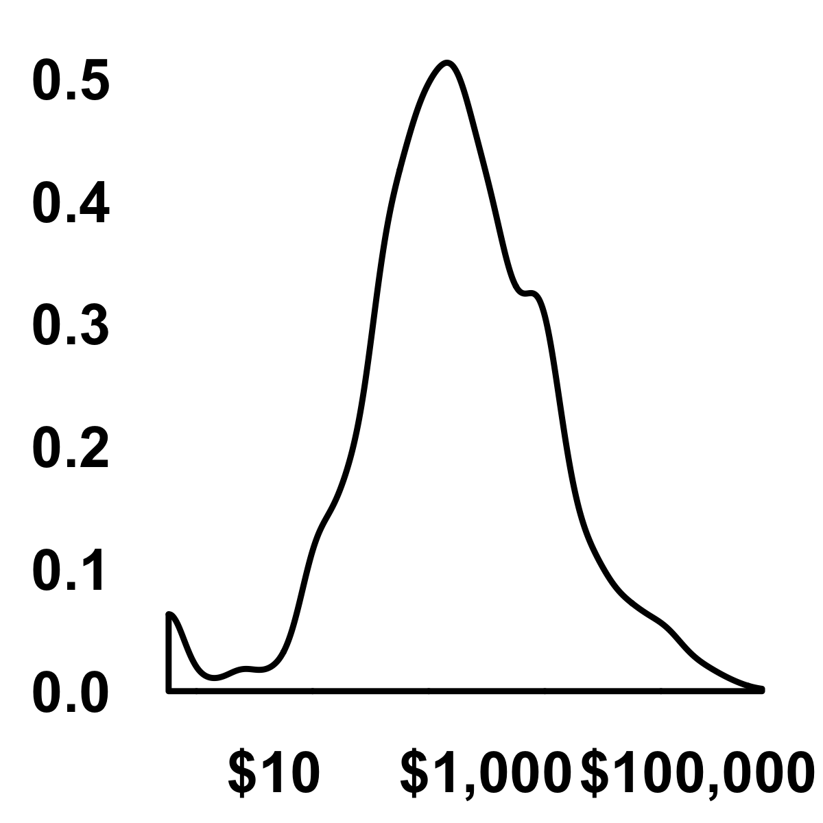
FIGURE 11.1: Density distribution
11.2 Create Quintiles
Once you have the summary data, you would like to put these donors in bins. Typically, each measure is divided into five bins. The top 20% of each measure go in bin number five and the bottom 20% go in bin number one. If a donor is in the top 20% for each of the measures, then his or her RFM score will be 555. Similarly, if a donor is in the bottom 20% for each of the measures, then his or her RFM score will be 111. We can use the ntile function from the dplyr library to compute these percentile bins.
rfm_ranks <- rfm_counts %>%
  mutate_at(.funs = funs(rank = ntile(., n = 5)),
            .vars = vars(Frequency, Monetary)) %>%
  mutate(Recency_rank = 5 - Recency) %>%
  mutate(RFM_score = as.integer(paste0(Recency_rank,
                                       Frequency_rank,
                                       Monetary_rank)))

glimpse(rfm_ranks)
#> Observations: 3,058
#> Variables: 8
#> $ ID             <int> 1, 2, 3, 4, 5, 7, 8, 9...
#> $ Recency        <dbl> 0, 0, 0, 0, 3, 3, 2, 0...
#> $ Frequency      <int> 2, 5, 4, 3, 2, 2, 2, 4...
#> $ Monetary       <dbl> 1600, 1585, 2930, 1725...
#> $ Frequency_rank <int> 2, 5, 5, 4, 2, 2, 2, 5...
#> $ Monetary_rank  <int> 4, 4, 5, 4, 4, 4, 3, 4...
#> $ Recency_rank   <dbl> 5, 5, 5, 5, 2, 2, 3, 5...
#> $ RFM_score      <int> 524, 554, 555, 544, 22...
head(rfm_ranks)
#> # A tibble: 6 x 8
#>      ID Recency Frequency Monetary Frequency_rank
#>   <int>   <dbl>     <int>    <dbl>          <int>
#> 1     1       0         2     1600              2
#> 2     2       0         5     1585              5
#> 3     3       0         4     2930              5
#> 4     4       0         3     1725              4
#> 5     5       3         2     1555              2
#> 6     7       3         2     1250              2
#> # ... with 3 more variables: Monetary_rank <int>,
#> #   Recency_rank <dbl>, RFM_score <int>
Here’s what the code is doing.
- The
mutate_atfunction is creating five bins for the Frequency and Monetary variables in the data. It is also creating a new variable using those variables with_rankas a suffix. Recency_rank = 5 - Recencyis creating a new variable by subtracting the current recency value from 5. We are doing so because the recency of a gift from 2016 will be zero, but it also needs the highest rank. What if you had actual gift dates? In that case, you would simply use thentilefunction to create five bins, but you would have to usedescbecause the latest gift date will have the lowest value and we want that value to have the highest bin number. You would use:mutate(Recency_rank = ntile(desc(Recency), 5)).- The last
mutatecall is simply concatenating the individual RFM bin numbers.
Let’s see what the giving looks like for the recency and frequency bins.
rfm_ranks %>% group_by(Recency_rank) %>%
  summarize(median(Monetary))
rfm_ranks %>% group_by(Frequency_rank) %>%
  summarize(median(Monetary))
As you can see from Table 11.2 and 11.3, for the top 20% of most recent and frequent donors, the median giving is higher than the other bins.
| Recency_rank | median(Monetary) |
|---|---|
| 1 | 100 |
| 2 | 222 |
| 3 | 330 |
| 4 | 506 |
| 5 | 755 |
| Frequency_rank | median(Monetary) |
|---|---|
| 1 | 114 |
| 2 | 200 |
| 3 | 432 |
| 4 | 836 |
| 5 | 1605 |
11.3 Plot Ranks
We can uncover various patterns when we visualize the RFM scores and ranks. Kohavi and Parekh (2004) shared different ways to look at these scores and ranks. Let’s look at a few, but please note that these visualizations are exploratory, thus I’m spending minimal time to make them pretty.
Let’s look at simple counts first. How many donors do we have in each of the bins? Figure 11.2 shows that a majority of the donors are in the 555 bin and some are in 111.
ggplot(rfm_ranks, aes(x = RFM_score)) +
  geom_bar() +
  theme_bw(base_size = 12)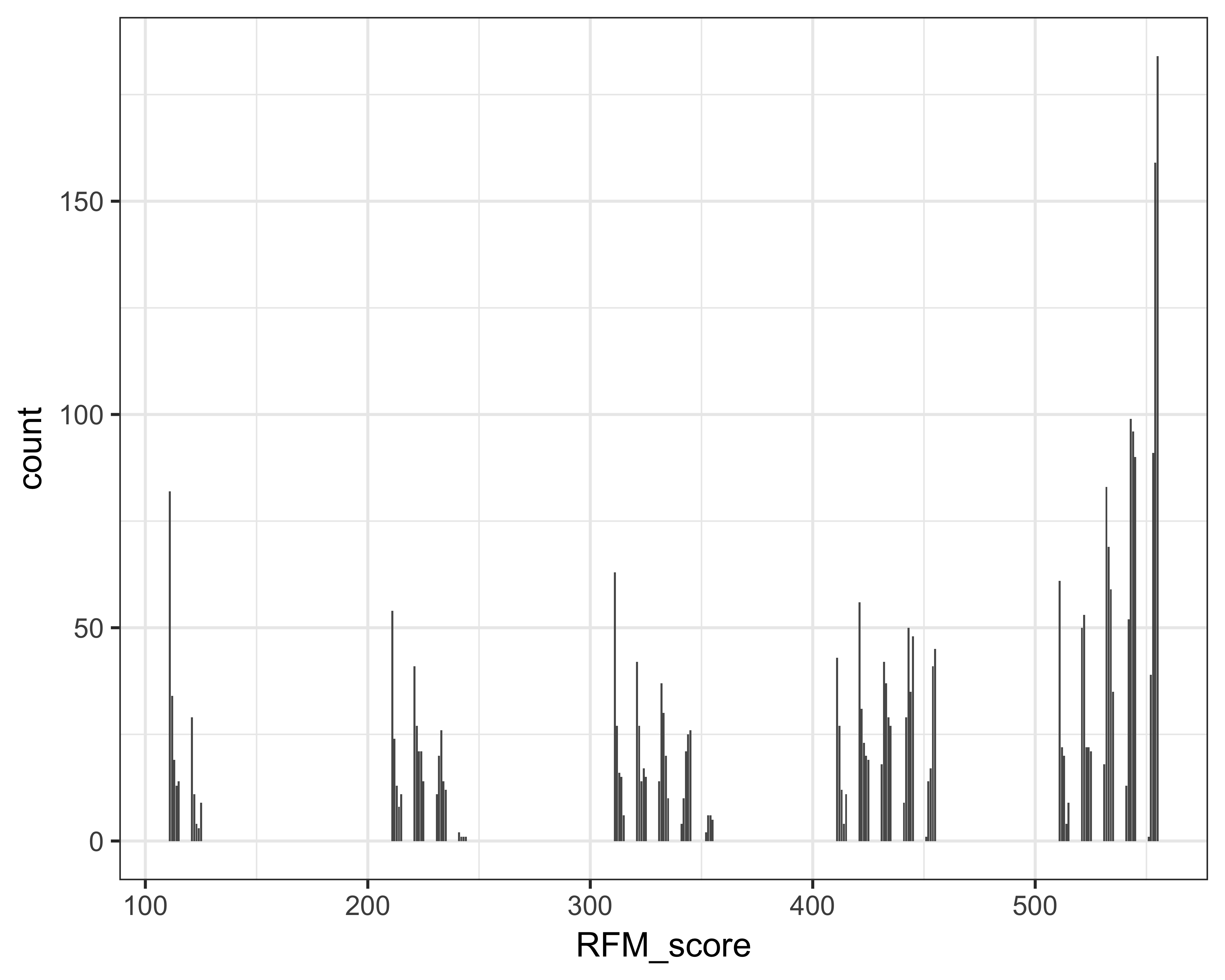
FIGURE 11.2: RFM scores and counts
Figure 11.3 shows, as suspected, that the donors with scores above 500 have higher giving. But some donors in the 300 range also have relatively higher giving. We should study this population because, although they have not given recently, they still have good frequency and have made large gifts.
library(ggplot2)
library(scales)

ggplot(rfm_ranks, aes(x = RFM_score,
                      y = Monetary,
                      size = Monetary,
                      color = factor(Monetary_rank))) +
  geom_jitter() + scale_colour_brewer() +
  scale_y_sqrt(labels = dollar) + theme_bw(base_size = 12) +
  theme(legend.position = "bottom")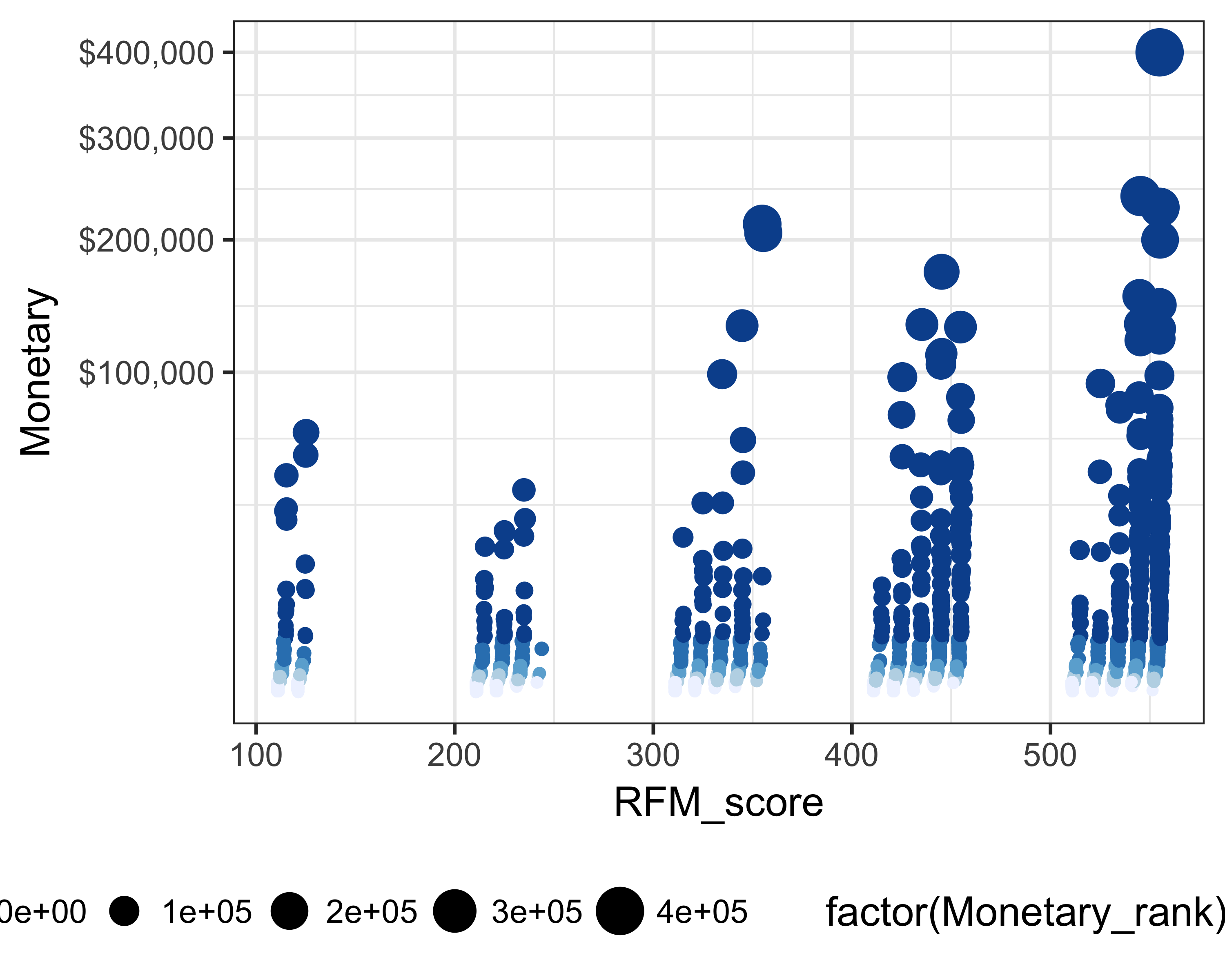
FIGURE 11.3: RFM scores and giving
Figure 11.4 shows the recency and frequency ranks and the giving values with circle sizes and color changes. You can see that the donors who don’t have recent gifts have not made frequent gifts either, although the gift size could be bigger.
ggplot(rfm_ranks, aes(x = Recency_rank,
                      y = Frequency_rank,
                      size = Monetary,
                      color = factor(Monetary_rank))) +
  geom_jitter() + scale_colour_brewer() +
  theme_bw(base_size = 12) +
theme(legend.position = "bottom") 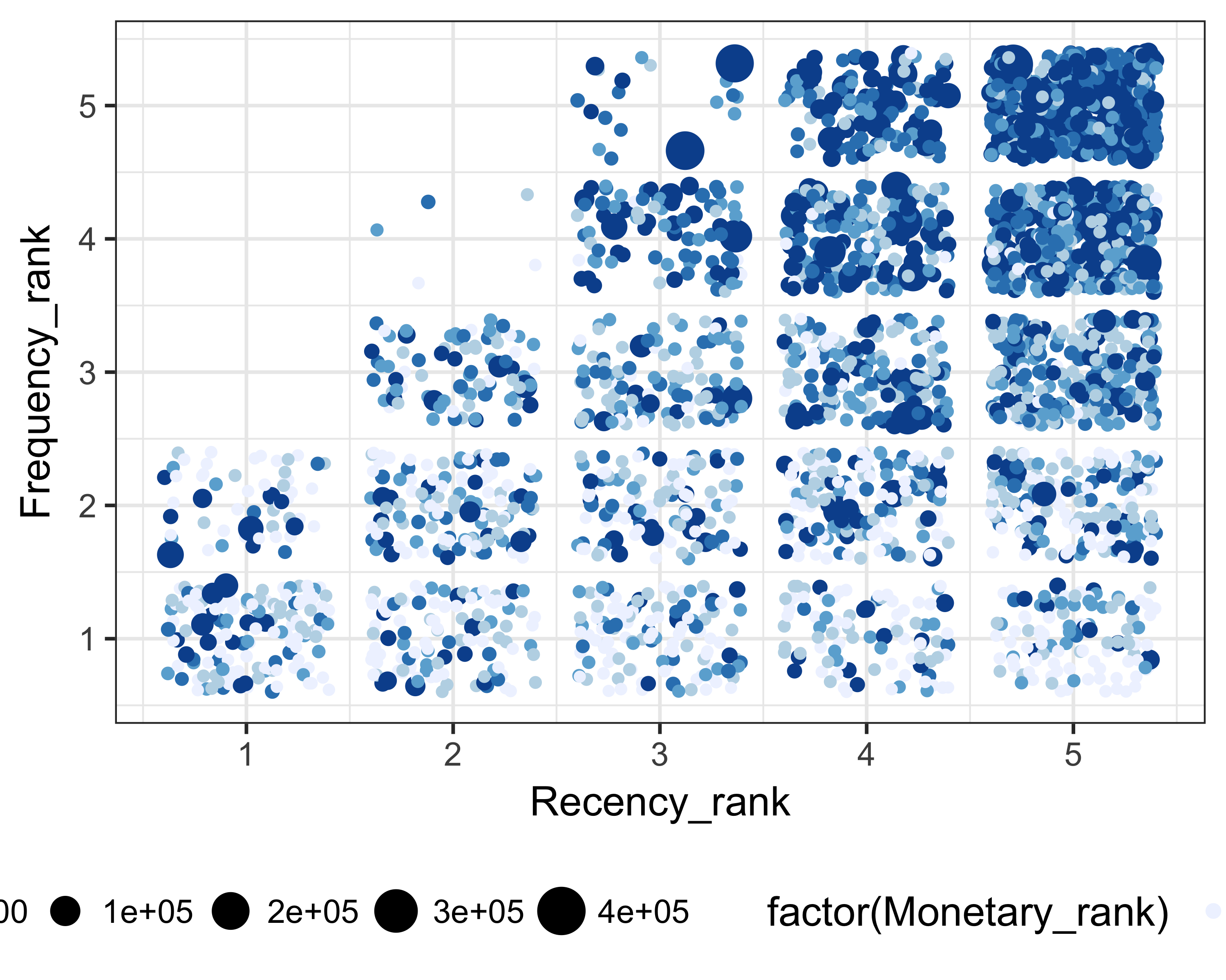
FIGURE 11.4: Recency rank, frequency rank, and giving
Figure 11.5 shows that donors who have given more frequently or recently tend to have slightly more giving (using median or 75th percentile as a measure).
ggplot(rfm_ranks, aes(x = factor(Frequency_rank), y = Monetary)) +
  geom_boxplot() + scale_y_sqrt(labels = dollar) +
  theme_bw(base_size = 12)
ggplot(rfm_ranks, aes(x = factor(Recency_rank), y = Monetary)) +
  geom_boxplot() + scale_y_sqrt(labels = dollar) +
theme_bw(base_size = 12) 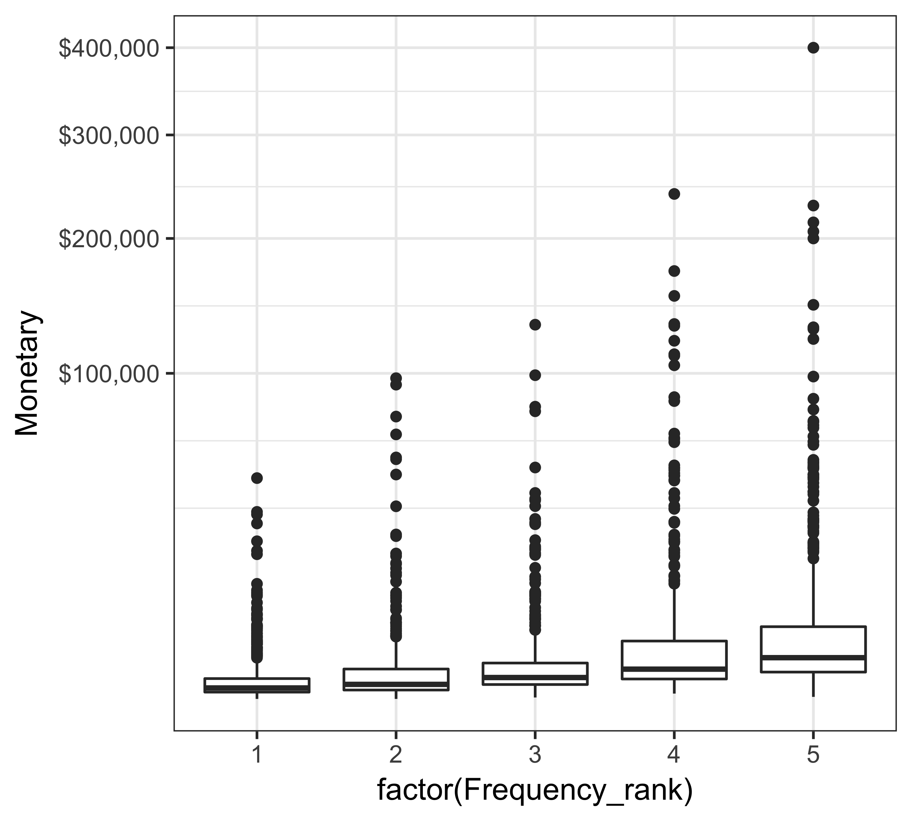
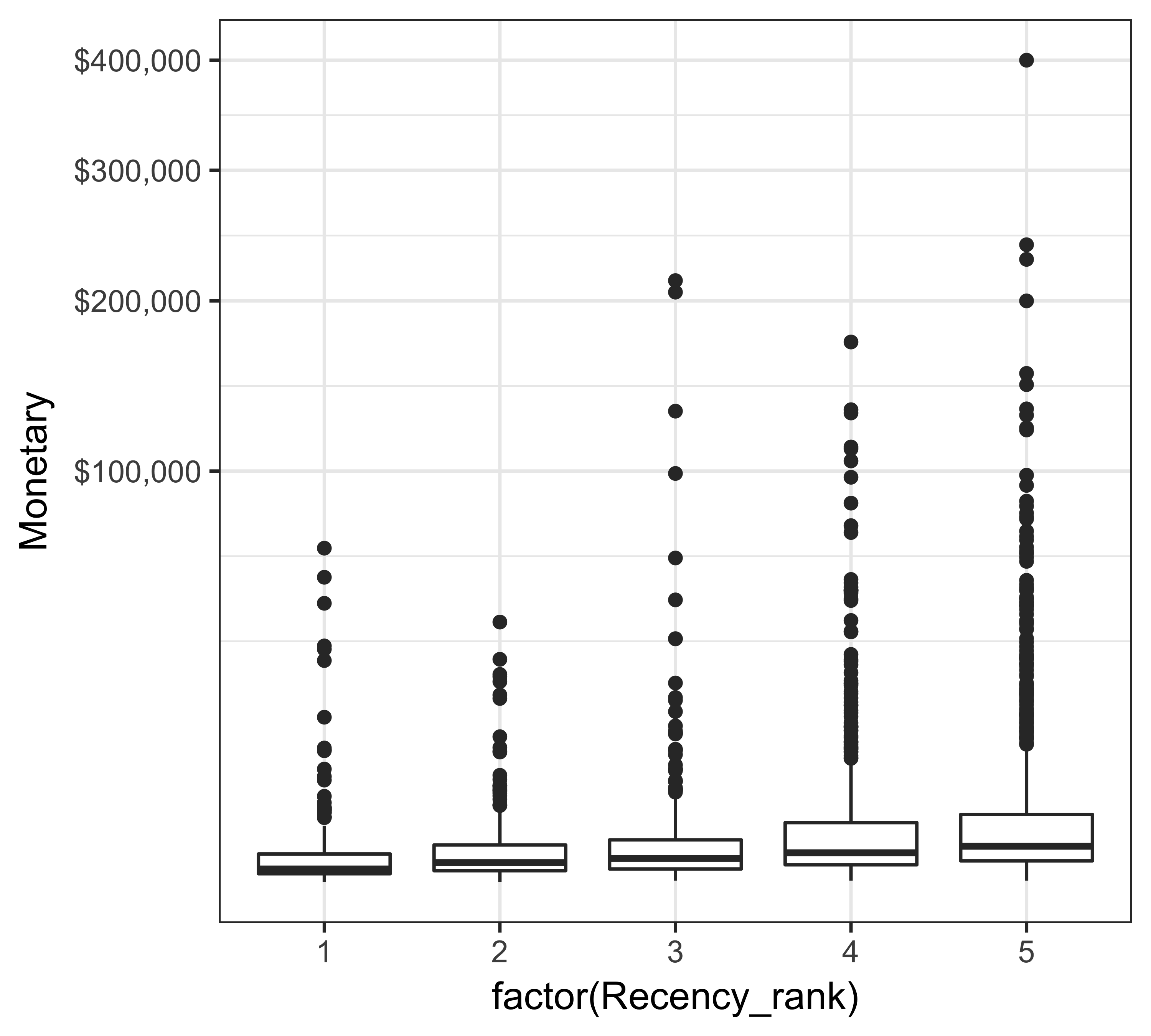
FIGURE 11.5: Box plot of giving
We can modify one of the plots used by Kohavi and Parekh (2004). In this plot, we show recency ranks on the X axis and frequency ranks on the Y axis. We then show the number of donors in each of the bins by changing the size of the points (shown as squares) and show the average giving by changing the color scale. Figure 11.6 shows the result of such a plot. It is clear from this plot that donors with a recency rank of three and frequency rank of five have the highest average giving as a group.
rfm_ranks %>%
  group_by(Recency_rank, Frequency_rank) %>%
  summarize(n = n(), avg_giving = mean(Monetary)) %>%
  ggplot(., aes(x = Recency_rank,
                y = Frequency_rank,
                fill = n))  +
  geom_tile(color = "white") +
  scale_fill_gradient(low = "#fed98e", high = "#993404") +
  theme_bw(base_size = 12) +
  theme(legend.position = "bottom")

rfm_ranks %>%
  group_by(Recency_rank, Frequency_rank) %>%
  summarize(n = n(), avg_giving = mean(Monetary)) %>%
  ggplot(., aes(x = Recency_rank,
                y = Frequency_rank,
                color = avg_giving,
                size = n))  + geom_point(shape = 15) +
  scale_color_gradient(low = "#fed98e", high = "#993404") +
  theme_bw(base_size = 12) + scale_size(range = c(5, 13)) +
  theme(legend.position = "bottom")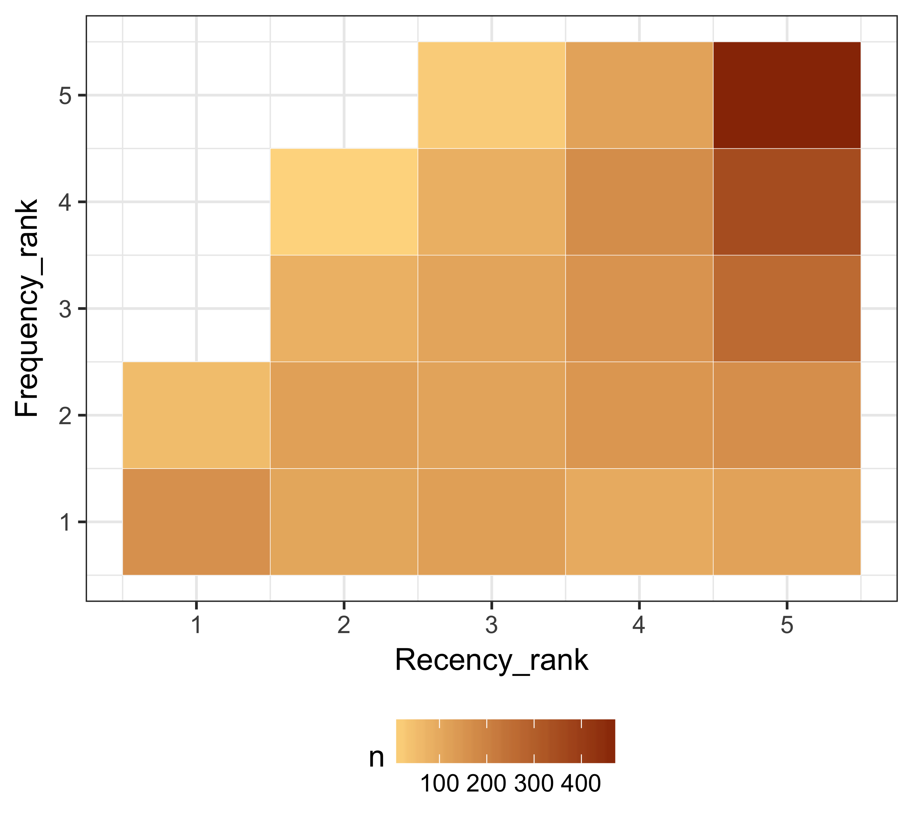
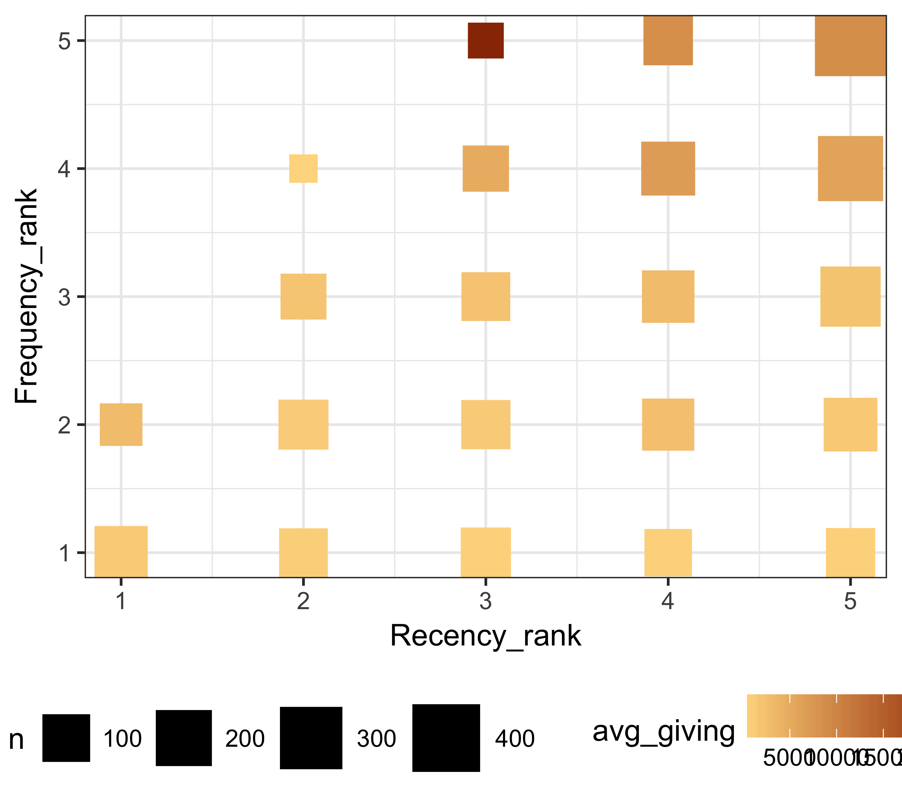
FIGURE 11.6: Recency and frequency rank along with giving
As a variation of Figure 11.6, in Figure 11.7, we can see the percentage of total donors that fall in each of these bins.
rfm_ranks %>%
  count(Recency_rank, Frequency_rank) %>%
  ungroup() %>%
  mutate(pct_donors = n / sum(n)) %>%
  ggplot(., aes(x = Recency_rank,
                y = Frequency_rank,
                fill = pct_donors,
                label = percent(pct_donors)))  +
  geom_tile(color = "white") +
  scale_fill_gradient(low = "white", high = "lightblue") +
  geom_text() + theme_bw(base_size = 12) +
  theme(legend.position = "bottom")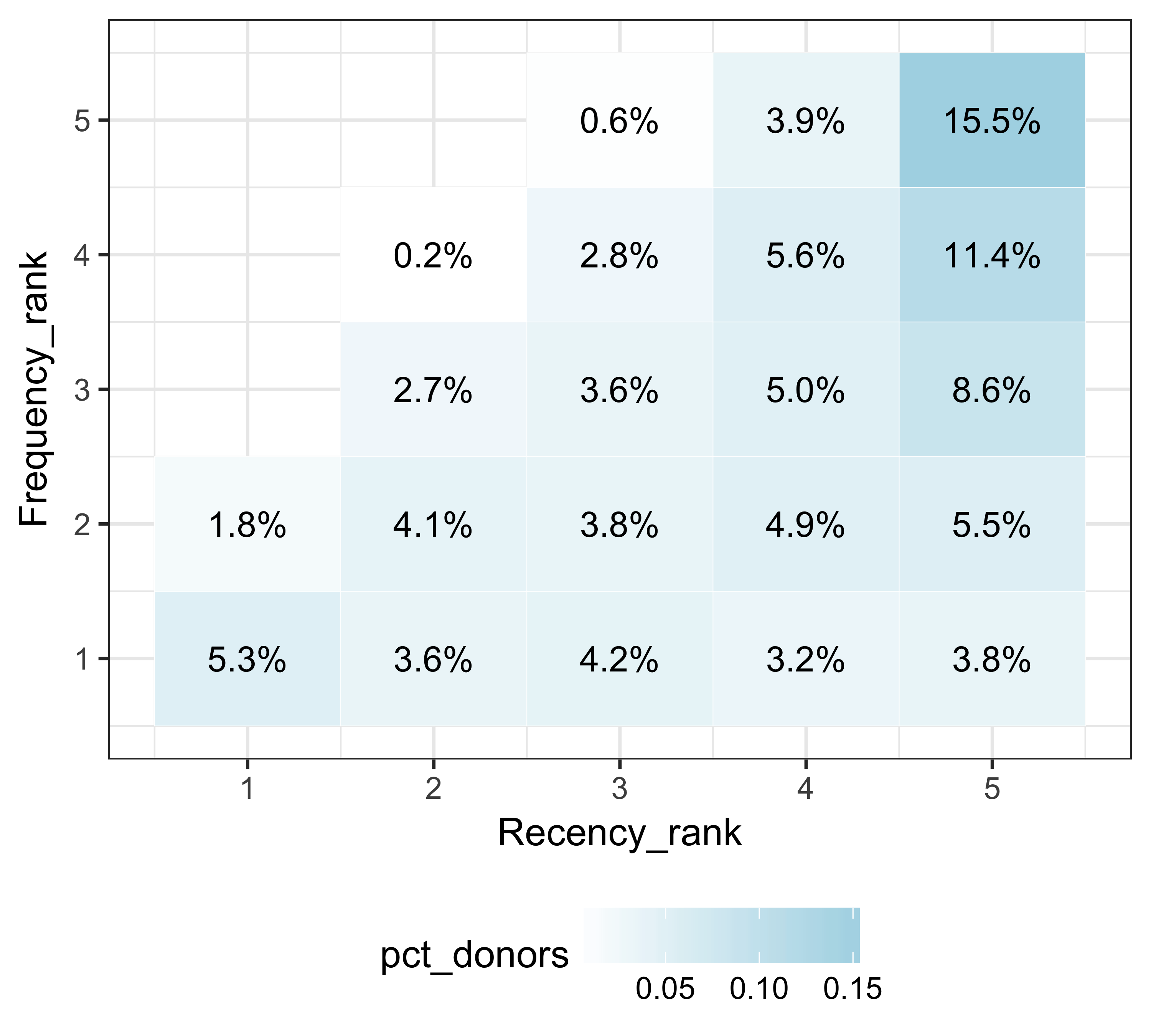
FIGURE 11.7: Recency and frequency rank along with giving
11.4 Use Cases
Let’s see some of the use cases of RFM scores and ranks:
- Find the future big donors: We can filter the 554 or 555 bins for any donors who have not given above a certain threshold. Since some donors in these bins have given large amounts, there’s a good likelihood that other donors may too. Let’s consider the average giving in these bins as the threshold.
avg_giving_555_554 <- mean(filter(
  rfm_ranks,
  RFM_score %in% c(555, 554))$Monetary)
filter(rfm_ranks, RFM_score %in% c(555, 554) &
         Monetary < avg_giving_555_554)
#> # A tibble: 280 x 8
#>      ID Recency Frequency Monetary Frequency_rank
#>   <int>   <dbl>     <int>    <dbl>          <int>
#> 1     2       0         5     1585              5
#> 2     3       0         4     2930              5
#> 3     9       0         4     1740              5
#> 4    19       0         5     4882              5
#> 5    22       0         4     3436              5
#> 6    32       0         4     3420              5
#> # ... with 274 more rows, and 3 more variables:
#> #   Monetary_rank <int>, Recency_rank <dbl>,
#> # RFM_score <int>- Upgrade donors: We can find the donors who have given recently and frequently but have not made large gifts. We can find such donors by looking at the 551 or 552 bins.
filter(rfm_ranks, RFM_score %in% c(551, 552))
#> # A tibble: 40 x 8
#>      ID Recency Frequency Monetary Frequency_rank
#>   <int>   <dbl>     <int>    <dbl>          <int>
#> 1   715       0         4      270              5
#> 2   736       0         4      229              5
#> 3   764       0         4      270              5
#> 4   852       0         4      192              5
#> 5  1003       0         4      136              5
#> 6  1283       0         4      276              5
#> # ... with 34 more rows, and 3 more variables:
#> #   Monetary_rank <int>, Recency_rank <dbl>,
#> # RFM_score <int>- Find cheaper channels for appeals: We don’t need to waste resources on donors who are not very likely to respond or make bigger gifts. We can find these donors by looking at bins 111, 112, 121, 122, 211, 212, 221, and 222.
filter(rfm_ranks, RFM_score <= 222 &
         !(substr(RFM_score, start = 3, stop = 3) %in% 4:5))
#> # A tibble: 338 x 8
#>      ID Recency Frequency Monetary Frequency_rank
#>   <int>   <dbl>     <int>    <dbl>          <int>
#> 1    33       3         1      500              1
#> 2    34       4         1        1              1
#> 3    35       4         1      150              1
#> 4    41       3         1       20              1
#> 5    78       4         1      320              1
#> 6    88       4         1      100              1
#> # ... with 332 more rows, and 3 more variables:
#> #   Monetary_rank <int>, Recency_rank <dbl>,
#> # RFM_score <int>- Re-acquire lapsed donors: Lapsed donors are very hard to re-acquire, but we may try reaching out to lapsed donors (recency rank < 4) who used to give frequently.
filter(rfm_ranks, RFM_score < 400 &
         (substr(RFM_score, start = 2, stop = 2) %in% 4:5))
#> # A tibble: 110 x 8
#>      ID Recency Frequency Monetary Frequency_rank
#>   <int>   <dbl>     <int>    <dbl>          <int>
#> 1    21       2         3      307              4
#> 2    45       2         3      871              4
#> 3    64       2         3     3887              4
#> 4    76       2         3     2260              4
#> 5   157       2         3   131303              4
#> 6   215       2         3     1345              4
#> # ... with 104 more rows, and 3 more variables:
#> #   Monetary_rank <int>, Recency_rank <dbl>,
#> # RFM_score <int>substr function. Write, test and run code in your console to find out the last letter of Iron Man.
If you’re enjoying this book, consider sharing it with your network by running
source("http://arn.la/shareds4fr")in yourRconsole.— Ashutosh and Rodger
References
McCarty, John A, and Manoj Hastak. 2007. “Segmentation Approaches in Data-Mining: A Comparison of Rfm, Chaid, and Logistic Regression.” Journal of Business Research 60 (6). Elsevier: 656–62.
Verhoef, Peter C, Penny N Spring, Janny C Hoekstra, and Peter SH Leeflang. 2003. “The Commercial Use of Segmentation and Predictive Modeling Techniques for Database Marketing in the Netherlands.” Decision Support Systems 34 (4). Elsevier: 471–81.
Yang, Amoy X. 2004. “How to Develop New Approaches to Rfm Segmentation.” Journal of Targeting, Measurement and Analysis for Marketing 13 (1). Springer: 50–60.
Kohavi, Ron, and Rajesh Parekh. 2004. “Visualizing Rfm Segmentation.” In Proceedings of the 2004 Siam International Conference on Data Mining, 391–99. SIAM.