Chapter 5 Getting Started with R

If you are completely new to all things R, welcome!

If you have a background in computer programming languages or software such as Python, Stata®, SAS®, or Matlab®, you may notice many familiar concepts and terminology such as functions, variables, and operators in the example R code recipes referenced in this book.

5.1 Why R?

R is a free, open source statistical programming language that is powerful, flexible, and evolving. R, which has grown significantly in popularity, is an interactive and object-oriented programming language that offers a variety of data structures, graphical capabilities, functions, packages, documentation, and community support. In addition, it is an evolving ecosystem that can effectively handle different data types and perform complex analysis on individual and distributed computer systems, which are important capabilities to consider when developing data analytics solutions of any size or scale.

5.2 Download R (Required)

R is compatible with Windows™, macOS, and a variety of Unix systems.

The latest version of R is available for download via the Comprehensive R Archive Network (CRAN):

• https://cran.r-project.org/

All of the R code in this book has been tested to work with R version 3.5.2 (2018-12-20). Please check your existing R installation and upgrade to the latest version if needed.

Remember to download all the R code files and data by visiting http://www.nandeshwar.info/ds4fundraisingcode.

5.3 Install RStudio (Optional)

RStudio is an integrated development environment (IDE), which includes a code editor, debugger, and visualization tools that make R more user friendly.

RStudio Desktop (Open Source Edition) is available for free download via the following links:

• RStudio: https://www.rstudio.com/

• RStudio Desktop: https://www.rstudio.com/products/rstudio/#Desktop

5.4 Install Packages

R is a popular programming language that benefits from community-driven support and ongoing enhancements.

R packages, which you may have already heard about, are bundles of reusable R functions, support documentation, and sample data (if included). As of writing this book, there are currently 12,106 R packages available to download, install, and use. The fact that there are over 12,000 packages of freely available add-on code libraries speaks to the flexibility of the R language and the robust commitment of the R user community. The potential data analytics solutions you can develop using these packages is perhaps only limited by your curiosity, creativity, and willingness to learn R!

We assume you’ve already downloaded R on your computer, so now it’s time to get your feet wet and download two popular R packages, dplyr and ggplot, using the install.packages function to familiarize yourself with the R package installation process.

To run the following code, copy and paste each line into your R console window and click the Enter key. Alternatively, you can copy and paste these commands into a new R script by selecting File > New File > R Script within R Studio.

# Install dplyr package
install.packages("dplyr", repos='http://cran.us.r-project.org')

# Install ggplot2 package
install.packages("ggplot2", repos='http://cran.us.r-project.org')

Voila! You successfully ran your first R code, which downloaded and installed two popular R packages for data manipulation and visualization tools. We’ll cover these tools later in greater detail.

These lines of R code contain two install.packages commands, each of which is preceded by a comment line indicated by the # symbol. The # symbol is a comment symbol that will not be executed by R. As a good programming practice, comment your code liberally to document it for later reference.

We strongly recommend you get into the habit of documenting your code with comment lines using the # symbol so that you can later reference, check, test, and update your code as needed.

If you create a new R script, you can also highlight all four lines of code in your script with your mouse cursor and then manually select Code > Run Select Line(s) from the R Studio menu. Alternatively, you can use the keyboard shortcut Command + Enter on a Mac or Control + Enter on Windows or Linux to run these lines of code.

For a full list of RStudio keyboard shortcuts, please refer to RStudio’s knowledge base.

Now that you’ve installed both R packages, let’s load these packages and make them available for use on your system using the library("package name") function.

# Load dplyr package
library("dplyr")

# Load ggplot2 package
library("ggplot2")

To see all of the R packages installed on your system, call the library function without any arguments (that is, inputs) or package names.

# List all packages installed
library()

In the library function output, you should see both the dplyr and ggplot2 packages listed in alphabetically along with the following brief package descriptions.

• dplyr: A Grammar of Data Manipulation

• ggplot2: Create Elegant Data Visualizations Using the Grammar of Graphics

Congratulations!

You just completed an R package installation process using repeatable and reusable R code, which downloaded, installed, and loaded R packages on your computer.

5.5 Learning R

Although R is a powerful statistical modeling and programming environment, it can take some time to get comfortable using R, especially if you don’t have any background in statistics or computer programming. For users with minimal experience in writing code, we encourage you to be patient while you get the hang of working with R. The benefits (flexibility, extensibility, and speed, just to name a few) are well worth the time and effort to overcome the initial learning curve associated with R.

Here are some tips for learning R:

• Do: Many people learn R best through hands-on learning and directly entering R commands within the R console window.
• Review: Check out code samples and retype the commands you find in this book and beyond.
• Experiment: Try modifying R commands and running the code to see what happens to develop a better sense and understanding of how it works.
• Research: You will encounter errors in R. Fortunately, R has excellent error messages that (usually) offer useful diagnostic information to help you figure out the root cause of the issue.

5.6 R Console

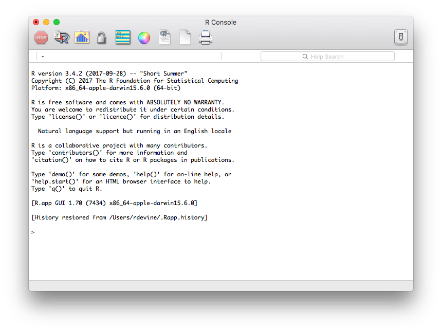
Assuming you’ve already installed R on your computer, the first thing you will encounter when you launch R is the R console window and the command prompt >, which indicates R is ready for your instructions.

FIGURE 5.1: Command prompt

As previously mentioned, R is an interactive programming environment, so let’s use R as a calculator and enter some basic arithmetic operators to explore it can do.

# Addition
1+8
#> [1] 9
# Subtraction
1-7
#> [1] -6
# Division
1/7
#> [1] 0.143
# Multiplication
1*7
#> [1] 7
# Exponentiation
2^3
#> [1] 8
# Order of Operations
1+2*3
#> [1] 7

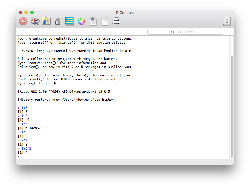
After you enter each command into the R command prompt, each result will be interactively displayed in the R console as shown in Figure 5.2.

FIGURE 5.2: Interactive output

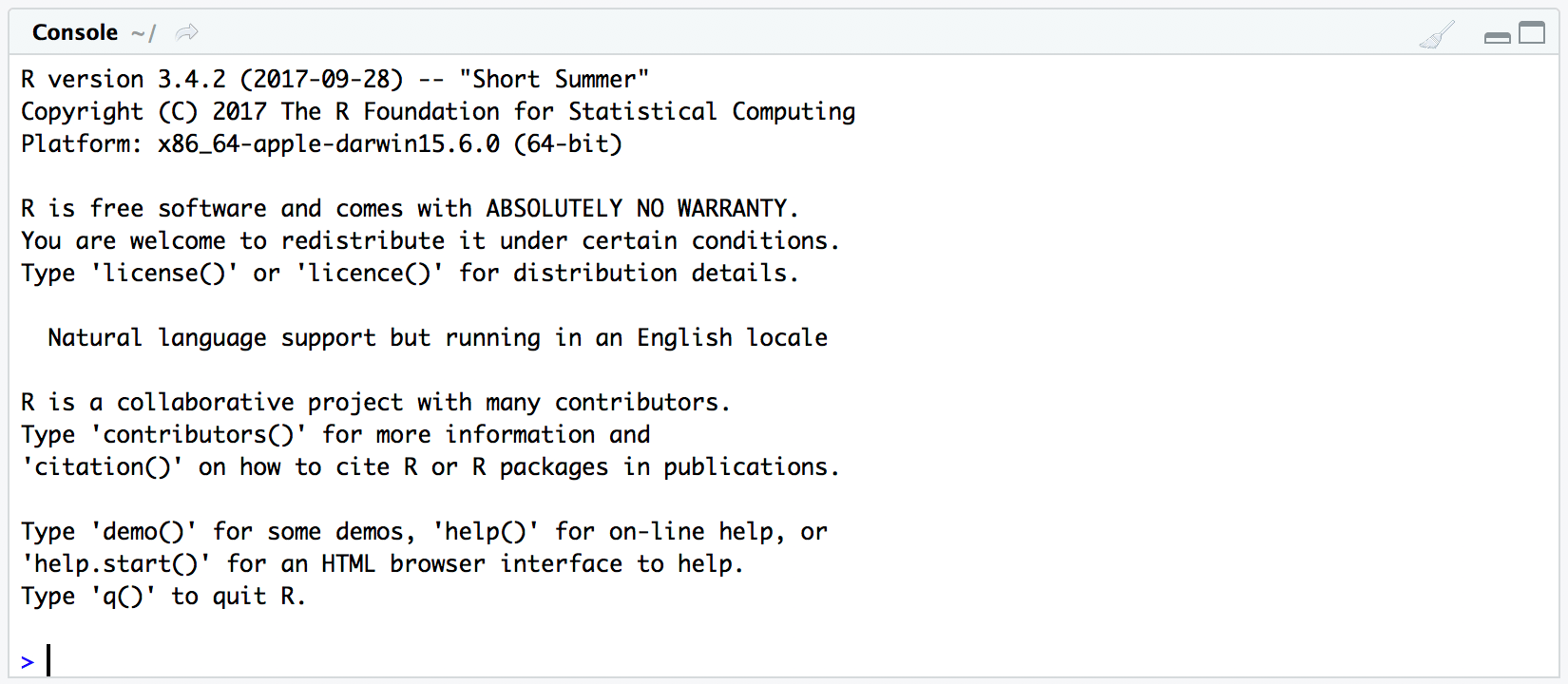
If you’ve installed RStudio, the R Console command prompt and interactive output will be displayed at the bottom of your RStudio session window.

FIGURE 5.3: RStudio command prompt

FIGURE 5.4: RStudio interactive output

5.7 Built-in Functions

R has many built-in functions, which are reusable expressions that involve zero or more variables.

# Logarithm
log(x = 100)
#> [1] 4.61
# Square Root
sqrt(x = 16)
#> [1] 4
# Round
round(x = 8.3)
#> [1] 8

These variables are arguments (inputs or parameters) that are passed to functions in order to perform various types of calculations. For example, the sqrt function takes a single argument of x. We used 16 as our x and the function returned its square root of 4.

Functions can also take more than one parameter, separated by commas.

In the previous example, the round function took the number 8.3 and rounded to the closest integer, which is 8. However, if we pass the round function a number such as pi (3.141592…), we can instruct R to round pi to the nearest hundredth by passing an additional parameter digits the value of 2.

# Round
round(x = 3.141592, digits = 2)
#> [1] 3.14

The base installation of R includes several built-in constant variables, one of which is pi.

• LETTERS: The 26 upper-case letters of the Roman alphabet
• letters: The 26 lower-case letters of the Roman alphabet
• month.abb: The three-letter abbreviations for the English month names
• month.name: The English names for the months of the year
• pi: The ratio of the circumference of a circle to its diameter

Rather that manually typing the value of pi in the previous example, you could have also used the built-in constant pi.

# Round
round(x = pi, digits = 2)
#> [1] 3.14

If you want additional information about a function and its parameters, the base R installation comes with useful help pages with function descriptions, usage, arguments, details, and examples.

You can view a function’s help documentation by using the ? operator or help function. Another way is using example(function_name) command. Try example(round) in your console.

To learn more about the round function and its usage details, try entering either of the following commands in your R console.

# ? Operator Help
?round

# Help Function
help(round)

To learn more about built-in constants in the base R namespace, try entering either of the following commands.

# ? Operator Help
?Constants

# Help Function
help(Constants)

R also allows you to write your own functions. If you are curious or are already comfortable using built-in functions, we encourage you to explore and try creating your own custom functions. For additional details, you can check out this article.

5.8 Variables

Variables allow you to store data in a named object, whose values can later be retrieved and changed as needed. To create a variable in R, use the assignment operator “<-”" to assign data to a variable name.

For example, suppose we wanted to store the value of the square root calculation for later use. Here’s a code snippet that stores the calculation in a variable.

# Calculate square root and assign to "sqroot" variable
sqroot <- sqrt(16)

# Print "sqroot" value
sqroot
#> [1] 4

In this example, you will note that we selected sqroot as the variable name to avoid a naming conflict with the sqrt function. To further extend this example, suppose we needed to regularly update the sqrt function input value instead of hard-coding the value “16”. We can modify the code to use another variable for the input parameter.

# Square Root Function Input (Parameter)
input <- 16

# Calculate square root and assign to "sqroot" variable
sqroot <- sqrt(input)

# Print "sqroot" value
sqroot
#> [1] 4

5.9 Conditional Logic

R provides a variety of logical operators that return a value of TRUE or FALSE.

# Less Than
1 < 2
#> [1] TRUE

# Less Than or Equal To
2 <= 2
#> [1] TRUE

# Greater Than
1 > 2
#> [1] FALSE

# Greater Than or Equal to
2 >= 2
#> [1] TRUE

# Exactly Equal to
2 == 2
#> [1] TRUE

# Not Equal To
1 != 1
#> [1] FALSE

# Not X
X <- TRUE
!X
#> [1] FALSE

# X or Y
X <- FALSE
Y <- TRUE
X | Y
#> [1] TRUE

# X AND Y
X <- FALSE
Y <- TRUE
X & Y
#> [1] FALSE

# Test whether value of X is TRUE 
X <- FALSE
isTRUE(X)
#> [1] FALSE

5.10 Data Types

Everything in R is an object. R offers a variety of data types such as scalars, vectors, matrices, data frames, and lists.

5.11 Vectors

A vector is an ordered collection of atomic (integer, numeric, character, or logical) values. Vectors are one of the most common and basic data structures in R, so it is useful to familiarize yourself with them.

Vectors can be one of two different types: (1) atomic vectors and (2) lists.

All of the elements in a vector must have the same data type.

You can manually create a vector by using the c, or combine, function to combine a collection of data values. For example, suppose we needed to create a list of donor ages and store them in a variable called donor_age.

# Create donor_age vector
donor_age <- c(28, 32, 77, 57, 52, 41, 42, 49)

We can use the c function again to add additional elements to donor_age if needed.

# Update donor_age with additional donor age values
donor_age <- c(donor_age, 72, 68)

5.12 Sequences

You can also create vectors as a sequence of numbers using the seq function or using the “:” operator.

seq(from = 1, to = 10)
#>  [1]  1  2  3  4  5  6  7  8  9 10
series <- 1:10
series
#>  [1]  1  2  3  4  5  6  7  8  9 10
# check whether they give same results
identical(x = seq(1, 10), y = series)
#> [1] TRUE

5.13 Matrices

Matrices are a special type of atomic (integer, numeric, character, or logical) vector with dimensional attributes (rows and columns). By default, matrices are filled column wise.

5.14 Lists

A list is a special vector type where elements are not restricted to a single data type. Because the contents of a list can include a mixture of data types, lists are flexible data structures and sometimes referred to as generic vectors.

To create a list, use the list function.

# Update donor_age with additional donor age values
donor_name <- "John Smith"
donor_age <- 58
donor_city <- "San Francisco"
donor_lifetimegiving <- 14225
donor_profile <- list(donor_name, donor_age, 
                      donor_city, donor_lifetimegiving)
donor_profile
#> [[1]]
#> [1] "John Smith"
#> 
#> [[2]]
#> [1] 58
#> 
#> [[3]]
#> [1] "San Francisco"
#> 
#> [[4]]
#> [1] 14225

5.15 Factors

Factors are vectors used to represent categorical data labels.

Factors can be ordered or unordered and are especially useful when organizing and working with categorical data due to their speed and efficiency. Although factors look like character vectors, they are actually stored internally within R as integers, so you need to be careful when treating them like characters to avoid running into errors. It is also important to note that factors can only contain pre-defined label values, also known as levels.

donor_ind <- factor(c("no", "no", "yes",
                      "yes", "yes", "no",
                      "no", "yes", "yes",
                      "yes"))
donor_ind

Let’s use the table function to create a two-way frequency table that shows the count of donors versus non-donors using the donor indicator variable donor_ind we just created.

donor_ind <- factor(c("no", "no", "yes", 
                      "yes", "yes", "no",
                      "no", "yes", "yes", 
                      "yes"))
table(donor_ind)
#> donor_ind
#>  no yes 
#>   4   6

5.16 Data Frame

A data frame is a special kind of list where each element has the same length. Data frames are important in R because they are used frequently for storing tabular data for analysis.

In addition to length, data frames have additional attributes, such as rownames, which can be used to organize and annotate data labels, such as donor_id.

Let’s create a data frame using the donor_age and donor_ind vectors we just created.

donor_age <- c(28, 32, 77, 
               57, 52, 41, 42,
               49, 72, 68)
donor_ind <- factor(c("no", "no", "yes", 
                      "yes", "yes", "no", 
                      "no", "yes", "yes", 
                      "yes"))
dd <- data.frame(donor_age, donor_ind)
dd
#>    donor_age donor_ind
#> 1         28        no
#> 2         32        no
#> 3         77       yes
#> 4         57       yes
#> 5         52       yes
#> 6         41        no
#> 7         42        no
#> 8         49       yes
#> 9         72       yes
#> 10        68       yes

Let’s use the table function to display a frequency table of donor_age and donor_ind.

table(dd)
#>          donor_ind
#> donor_age no yes
#>        28  1   0
#>        32  1   0
#>        41  1   0
#>        42  1   0
#>        49  0   1
#>        52  0   1
#>        57  0   1
#>        68  0   1
#>        72  0   1
#>        77  0   1

5.17 Data Types

R provides several functions to examine the features of various data types such as:

• class: What kind of data object?
• type: What kind of data storage type?
• length: What is the length of the data object?
• attributes: What kind of metadata?
• str: What kind of data object and internal structure?

5.18 Additional Support

We encourage you to start where you are and embrace the learning curve you inevitably encounter when learning any type of new language, whether computer or human.

For reference, the following is a link to R manuals provided by the R Development Core Team as a learning resource.

• https://cran.r-project.org/manuals.html

The following is a list of R community support sites with knowledgeable and helpful R user forums, which can be a useful resource when you encounter questions or run into a technical hurdle.

• https://r-dir.com/community/forums.html

# Install dplyr package
#install.packages("dplyr")

# Install ggplot2 package
#install.packages("ggplot2")

# Install tidyverse
#install.packages("tidyverse")

# Load dplyr package
library("dplyr")

# Load ggplot2 package
library("ggplot2")